Whitepaper Review: How Shazam Works - Part 1

Shazam is a mobile app that allows you to identify any song in their database by recording the song using your phones microphone. However, before the advent of mobile device app stores, they offered diall in a phone number service that would recognise a song for you over the phone.

As it turns out, to achieve this, they had to create a novel method of differentiating between millions of songs in a way that is highly invariant to poor microphone quality and noise. This technique, or variants of it, can be used for the detection of any number of different detection problems in audio analysis from bird songs to potentially engine sounds.

I have particular interest in this technique for my project on Engine Fault Detection using Audio Analysis. I am attempting to determine vehicle health from audio alone.

In this article, I’m going to break down how Shazam works and discuss how this could be relevant to my project.

High Level Overview

The technique that Shazam came up with was a robust audio fingerprint. The fingerprint takes the loudest sound frequency at different time intervals. It does this for an entire song to create a unique fingerprint for that song.

This method can create the same fingerprint even if the song is recorded on a low quality microphone and the recording is highly compressed. This is because the unique points in the fingerprint are the points of the highest audio magnitude for that interval. These points are so loud that they will be audible even in settings with a lot of background noise or on poor quality microphones.

Algorithm

TLDR

Audio file -> FFT Spectrogram -> Find local maxima -> Fingerprint hashing -> Find matching hashes

Don’t worry if you don’t understand any of these steps, I’m going to explain them all in more detail.

1. Frequency Transform

If you want an intuitive visualisation of the Fourier Transform, you really can’t compete with 3Blue1Brown’s video: https://www.youtube.com/watch?v=spUNpyF58BY.

Fig 1 above shows an audio waveform plotted in the time domain. Any audio waveform captured from a microphone consists of many different audio signals interacting with each other. The audio waveform that is captured is in effect a sum of all of the different signal sources.

In the case of the waveform in Fig 1, I created the waveform from three different sine waves.

The Fourier Transform breaks the audio waveform into its constituent frequency components. It tells us what frequencies are present in the waveform and to what degree they contribute to the waveform.

In the Fourier Transform shown in Fig 3 above, we can see that the waveform consists of a large 1Hz component as well as smaller 2Hz and 3Hz components.

Discrete Fourier Transform Function

So what does the fourier transform actually calculate on a waveform?

The actual discrete Fourier Transform function looks like:

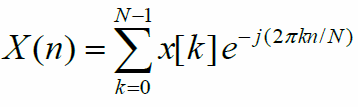
where:

• n is the nth frequency bin
• x[k] is the kth sample of the audio waveform
• N is the size of the window (ie the length of the waveform)

What is this function doing? Essentially, for each bin of frequencies we want to calculate the magnitude of, it iterates through every sample in the waveform and forms some weighted sum that represents the magnitude of the frequencies.

I mention frequency bin here and not frequency because in reality because we’re sampling the waveform, each frequency actually represents a range of frequencies of a size dependent on the number of samples.

How do we know the smallest bin size we can calculate? The frequency is the number of oscillations per second so we need to find out how many samples per second the waveform is sampled at and the total number of samples we have to sample the frequencies. For example, if our waveform was 4096 samples and it was sampled at 44.1kHz, the number of frequency bins would be: 44,100Hz/4096 = 10.76Hz per frequency bin.

Note that the the frequency resolution increases the longer the audio waveform is but the time resolution of the frequencies decreases.

2. Spectrogram

Windowed Fourier Transform

Fig 3 was a Fourier Transform taken over a 4-second clip. This means that it finds a sum of all of the frequency components present in the waveform. However, what if we wanted to find the frequency components present at each 1 second interval of the waveform?

We can calculate separate Fourier transforms for each second of audio. This technique is known as windowing. The problem now becomes how do we visualise the results. We now have reintroduced time as a dimension.

The answer is a spectrogram. It basically flips the fourier transform on its side and displays frequency magnitudes as colour intensities. It’s a pretty interesting way of visualising a waveform and is a great way of finding information hidden in the signal.

3. Spectrogram Filtering

So back to the context of Shazam, we have taken the audio of a potential song and created an interesting looking spectrogram of the song. Now we have to find an efficient method of identifying a unique song from this spectrogram.

The process needed to be noise tolerant so a natural first attempt was to find n frequencies with the highest magnitudes for each time slot in the spectrogram. This is because the loudest parts of a signal are the least effected by noise and should be possible to be identified even in very poor quality recordings.

There are issues with this approach however:

1. Human ears find it more difficult to hear lower frequencies. PA systems and song mixes are equalised to boost the low frequencies to counter this. Because of this, if you only take the most powerful frequencies, you will only have low frequency features.

2. Powerful frequencies on the spectrogram tend to cause adjacent frequency bins to falsely appear as powerful due to spectrum leakage (more on this later). If you only take the most powerful frequencies, you will have several adjacent bins as features.

The Shazam whitepaper doesn’t detail the actual algorithm that they use to calculate the features but several have been speculated. One I particularly like is:

1. For each FFT spectrogram result, split the frequency bins into logarithmically increasing frequency bands. For example if there were 512 frequency bins they would be split into:

• 0-10
• 10-20
• 20-40
• 40-80
• 80-160
• 160-511

2. Select the frequency bin with the highest magnitude in each band.

3. Compute the mean average magnitude of the band peaks.

4. Keep the peaks that fall above the magnitude average. This makes sure that only bands that are actually of high magnitude are kept and discards any bands that only contain noise.

Variables

The FFT parameters such as the number of bins and window size weren’t specified in the Shazam whitepaper and will require some experimentation to find an optimal approach. Also, although I mentioned using 6 bands here, any number of bands can be used to find optimal results.

Conclusion

This sums up how Shazam creates fingerprints of songs that can be used to identify the song from a recorded segment on a phone. In the second and final part of this algorithm review I am going to discuss how the fingerprints are used to search for the correct matching song efficiently.

References

[1] Shazam’s Whitepaper: https://www.ee.columbia.edu/~dpwe/pubs/OgleE07-pershash.pdf

[2] http://coding-geek.com/how-shazam-works/